4.6 Creating DSD, ContentConstraint and Dataflow
In SDMX, a Data Structure Definition (DSD) is used to organise data in a specific format. Represented as a cube, a DSD is made up of dimensions and attributes. A Dataflow, on the other hand, represents a specific portion or filtered view of the cube that the DSD represents. A Content Constraint specifies the permitted code list and codes for a particular Dataflow.
In SDMX Constructor, we can create DSDs, Dataflows and Concent Constraints either by “one by one” approach or in one go using the Table Modeller functionality.
We will first see how to apply the “one by one” approach and, subsequently, the Table Modeller functionality.
The “one by one” approach
Creating DSD
The following steps assume you already have a ConceptScheme created and the corresponding SDMX-ML (XML) file is saved on your computer.
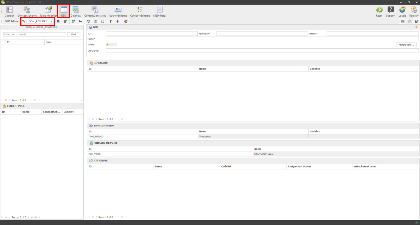
- Start the SDMX Constructor. Click on the DSD button in the Editor menu and ensure that the folder we created before, LOCAL_REGISTRY, is selected from the ‘Load from registry’ dropdown option, as shown below.
 Click here to enlarge the image
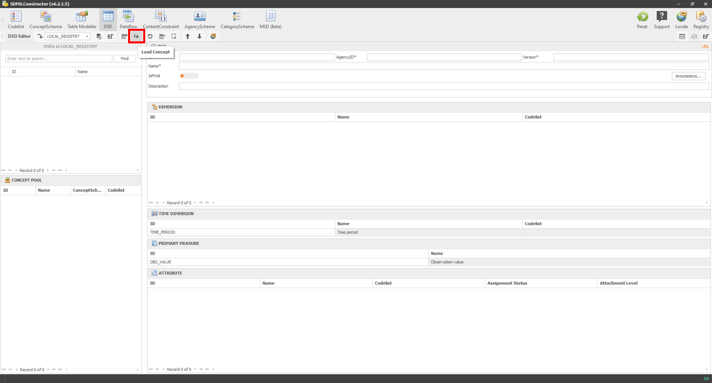
- Click on the ‘Load Concepts’ in the Editor Ribbon menu, as shown below.
 Click here to enlarge the image
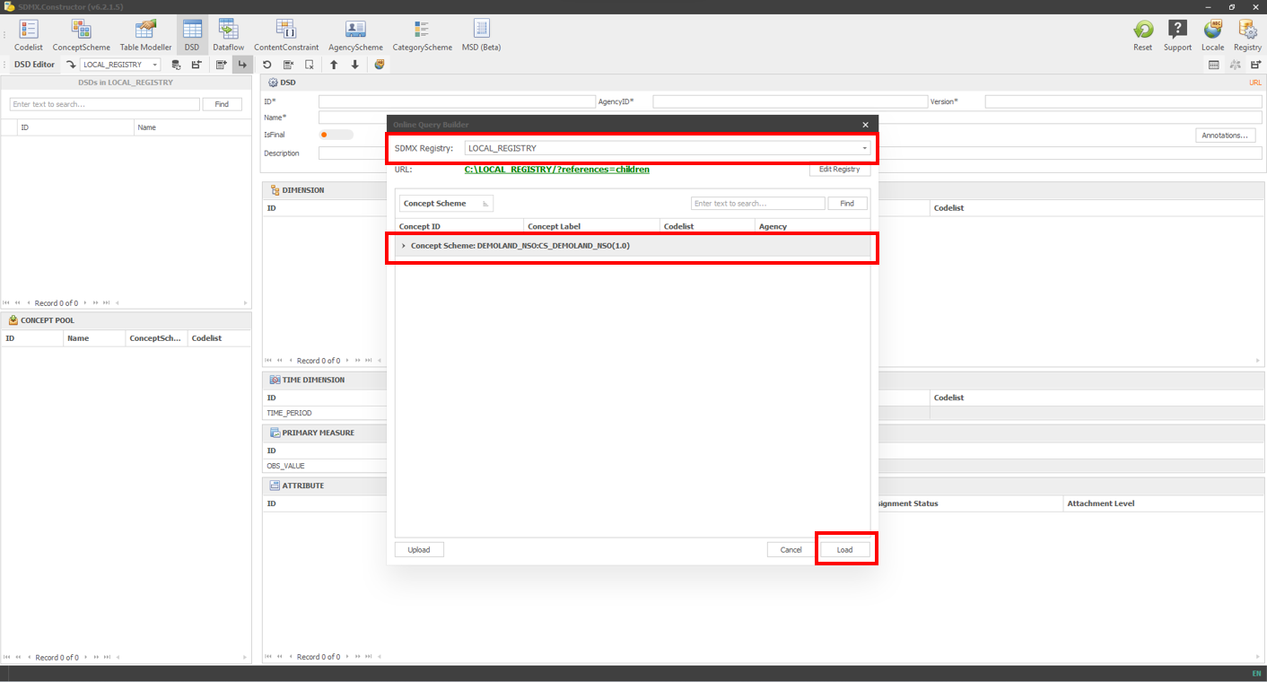
- In the resulting window, as shown below, select the SDMX Registry (which will be LOCAL_REGISTRY in this case). Then click on Load, as shown below.
 Click here to enlarge the image
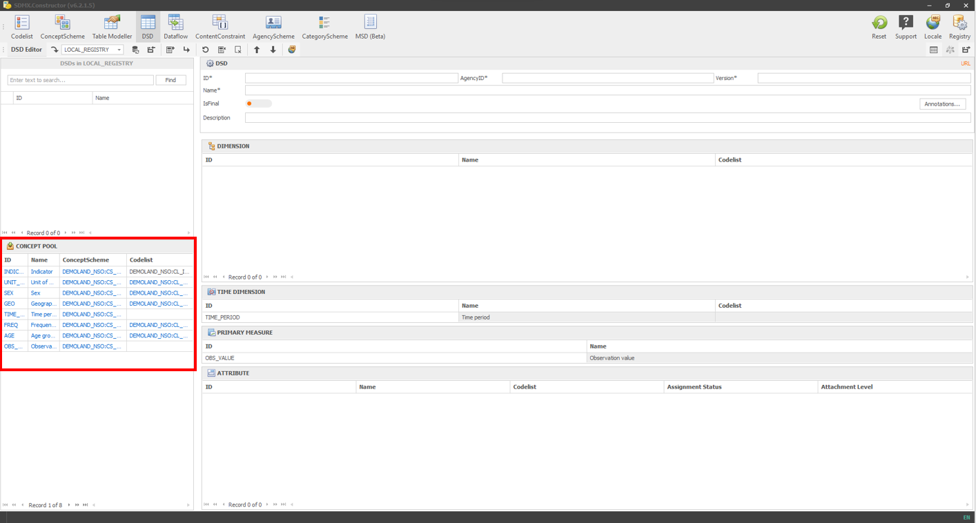
The concepts will be visible in the CONCEPT POOL, as shown below.
 Click here to enlarge the image
- Drag and drop the concepts from the CONCEPT POOL to either the DIMENSION or the ATTRIBUTE pane on the right. For our example data, except for the Unit of Measurement, which will go to the ATTRIBUTE pane, all other concepts will be in the DIMENSION pane, as shown below.
 Click here to enlarge the image
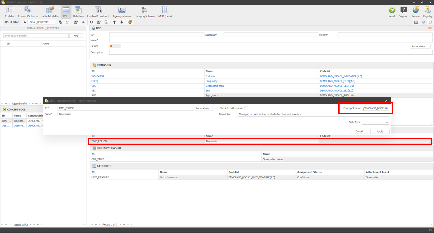
- Note that by default, SDMX Constructor has preselected TIME DIMENSION and PRIMARY MEASURE on the right pane. However, ensure that the ConceptScheme fields in both are set to the same (DEMOLAND_NSO:CS_DEMOLAND_NSO(1.0)) as other dimensions. Double-clicking the TIME DIMENSION will open up the pop-up window where it can be specified, as shown below. Click Apply.
 Click here to enlarge the image
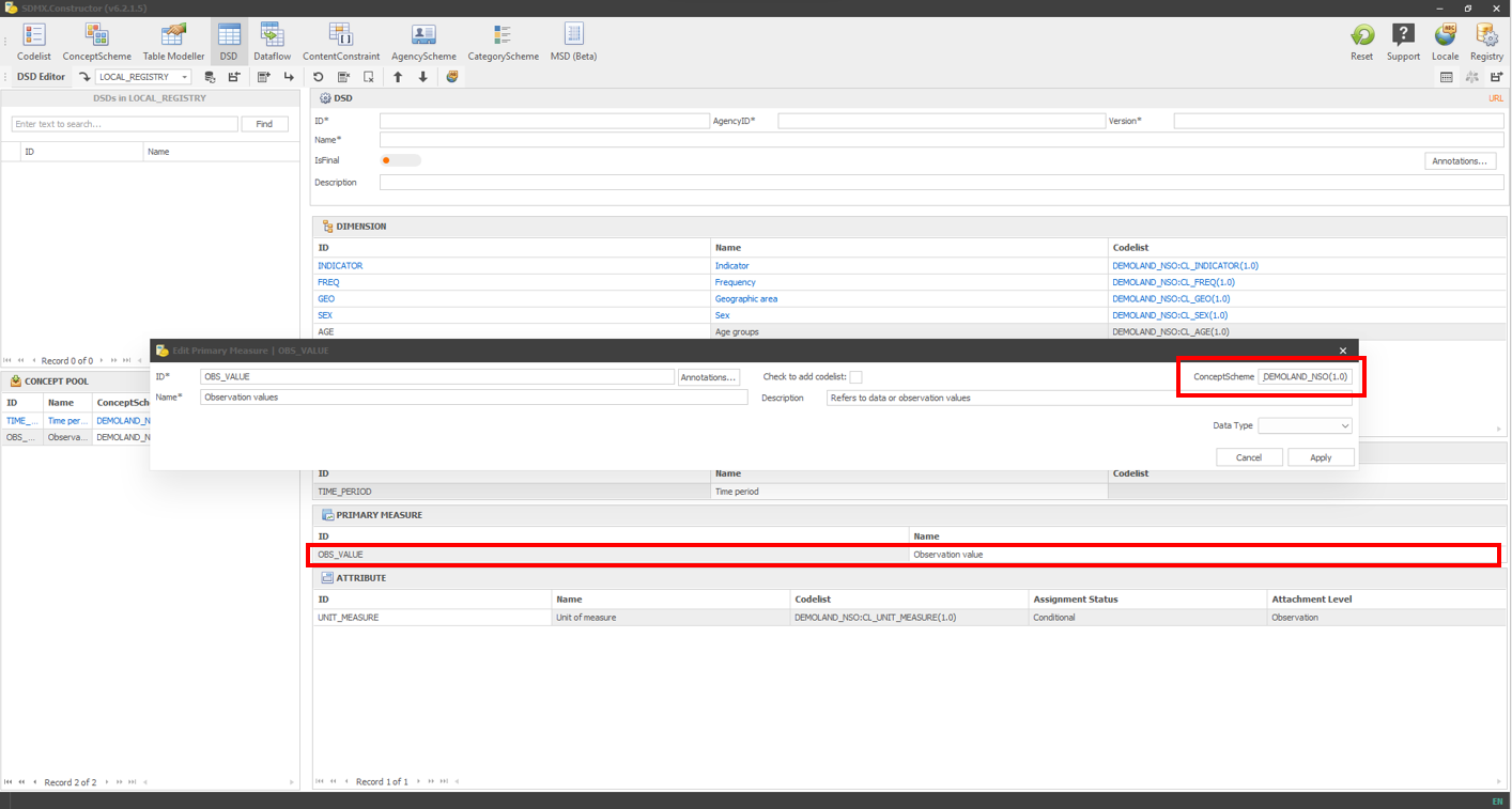
- Repeat the same for the PRIMARY MEASURE as shown below. Click Apply.
 Click here to enlarge the image
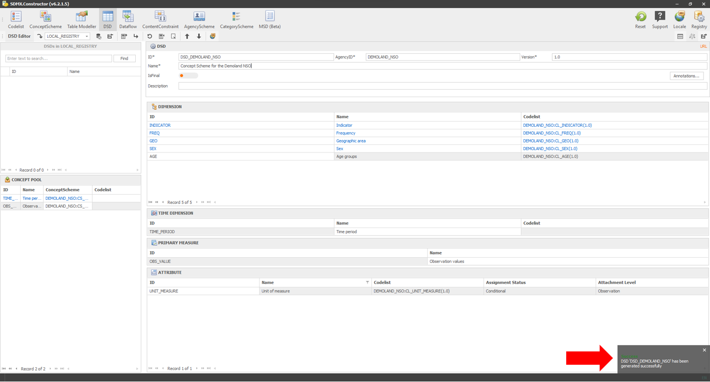
- Fill in the details for the DSD (ID = DSD_DEMOLAND_NSO, AgencyID = DEMOLAND_NSO, Version = 1.0 and Name = Concept Scheme for the Demoland NSO) as shown below.
 Click here to enlarge the image
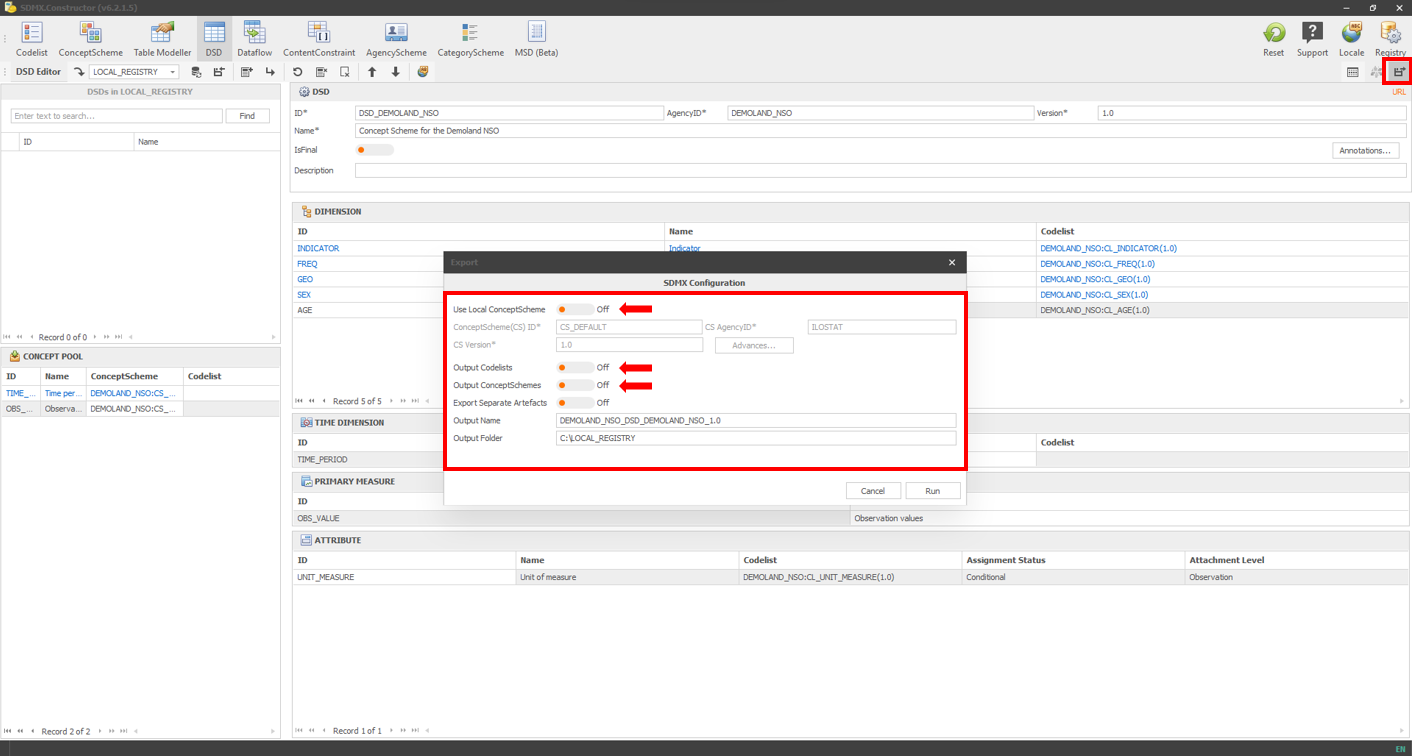
- Clicking on the Export/Save button, as shown below, will open up a pop-up window where you can make the following adjustments: Use Local ConceptScheme - turn it off; output Codelists - turn it off and Output ConceptSchemes - turn it off.
 Click here to enlarge the image
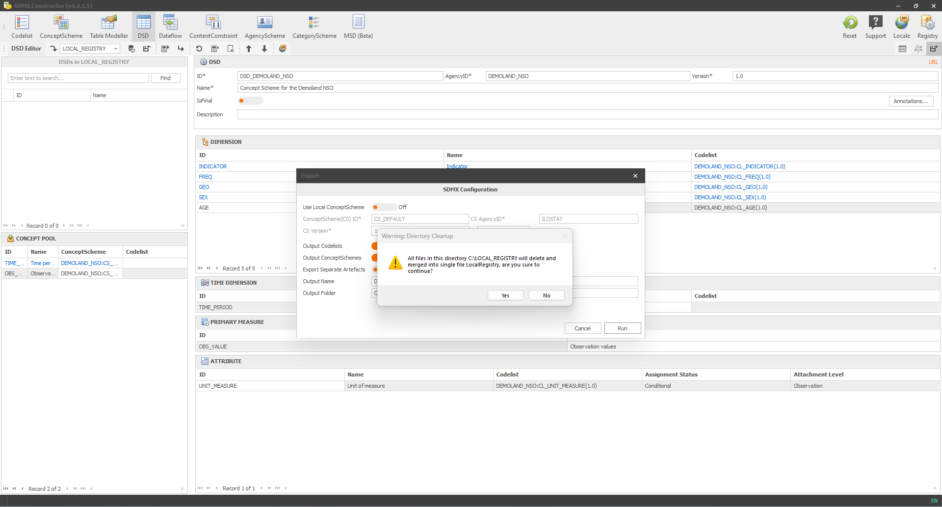
- Clicking on Run will show the following message. Click on Yes.
 Click here to enlarge the image
- You will see a message confirming the creation of the DSD, as shown below.
 Click here to enlarge the image
- After that, you will see the XML file created if you go to the file’s location.
Creating Dataflow
- Click on the Dataflow button in the Editor menu and ensure that the folder we created before, LOCAL_REGISTRY, is selected from the ‘Load from registry’ dropdown option, as shown below.
 Click here to enlarge the image
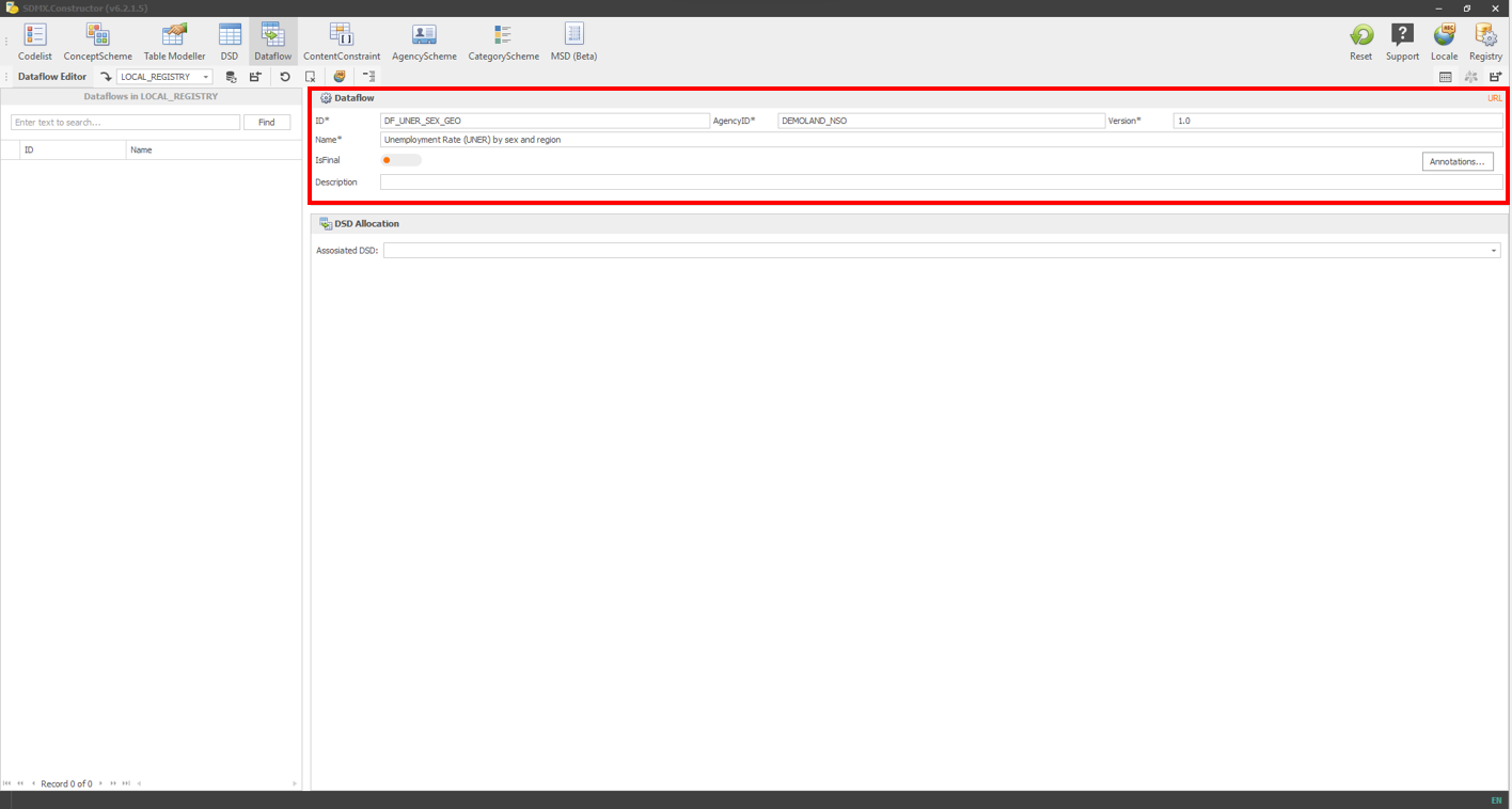
- For this example of Dataflow, we will select ‘Table 4.1: Unemployment Rate by sex and region’. We will first enter the details (ID = DF_UNER_SEX_GEO, AgencyID = DEMOLAND_NSO, Version = 1.0 and Name: Unemployment Rate (UNER) by sex and region) as shown below.
 Click here to enlarge the image
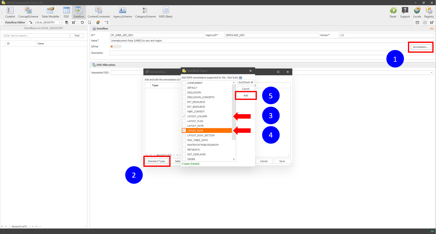
- Then click on the Annotation button. After that, click on Standard Types in the pop-up window. Then select the LAYOUT_COLUMN and LAYOUT_ROW from the list. Finally, click on the Add button, as shown below.
 Click here to enlarge the image
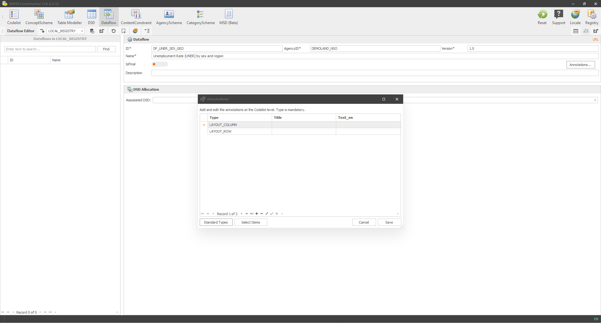
- You will see the following window.
 Click here to enlarge the image
- Select the LAYOUT_COLUMN. Then click in the Title column field. Then click on the Select Items button. Then following the layout scheme of Table 4.1, select the items for LAYOUT_COLUMN: as SEX and TIME_PERIOD. Finally, click on the Insert button.
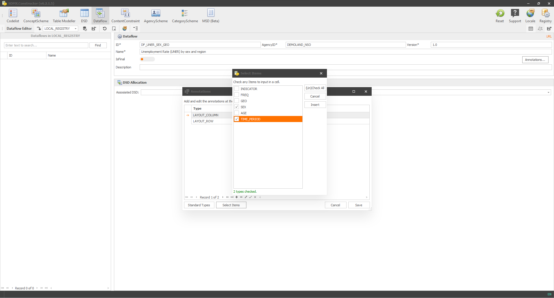 Click here to enlarge the image
- Repeat the same for the LAYOUT_ROW. Click inside the corresponding field of the column ‘Title’, then click on the Select Items button. Then select GEO (as per Table 4.1) and click on the Insert button.
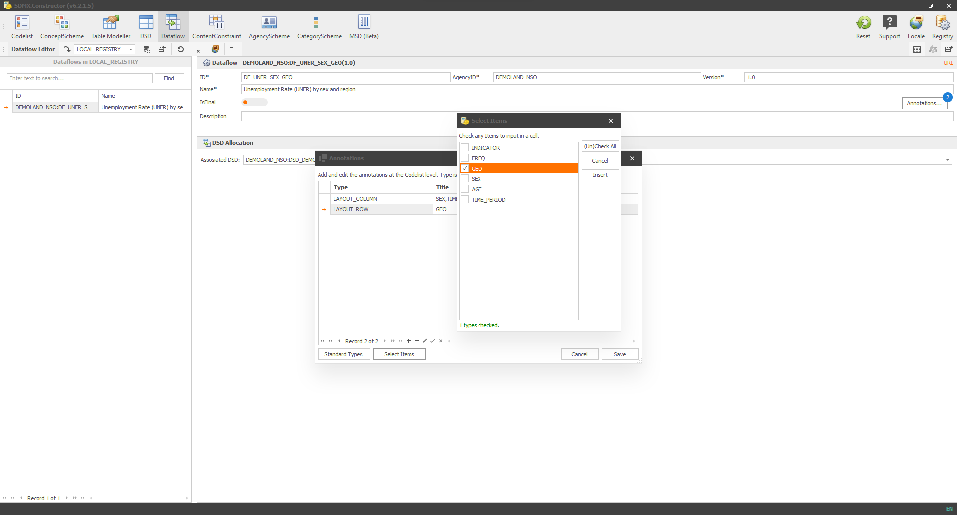 Click here to enlarge the image
- This is how it would look after both entries.
 Click here to enlarge the image
- Clicking on the Save button will result in the following confirmation.
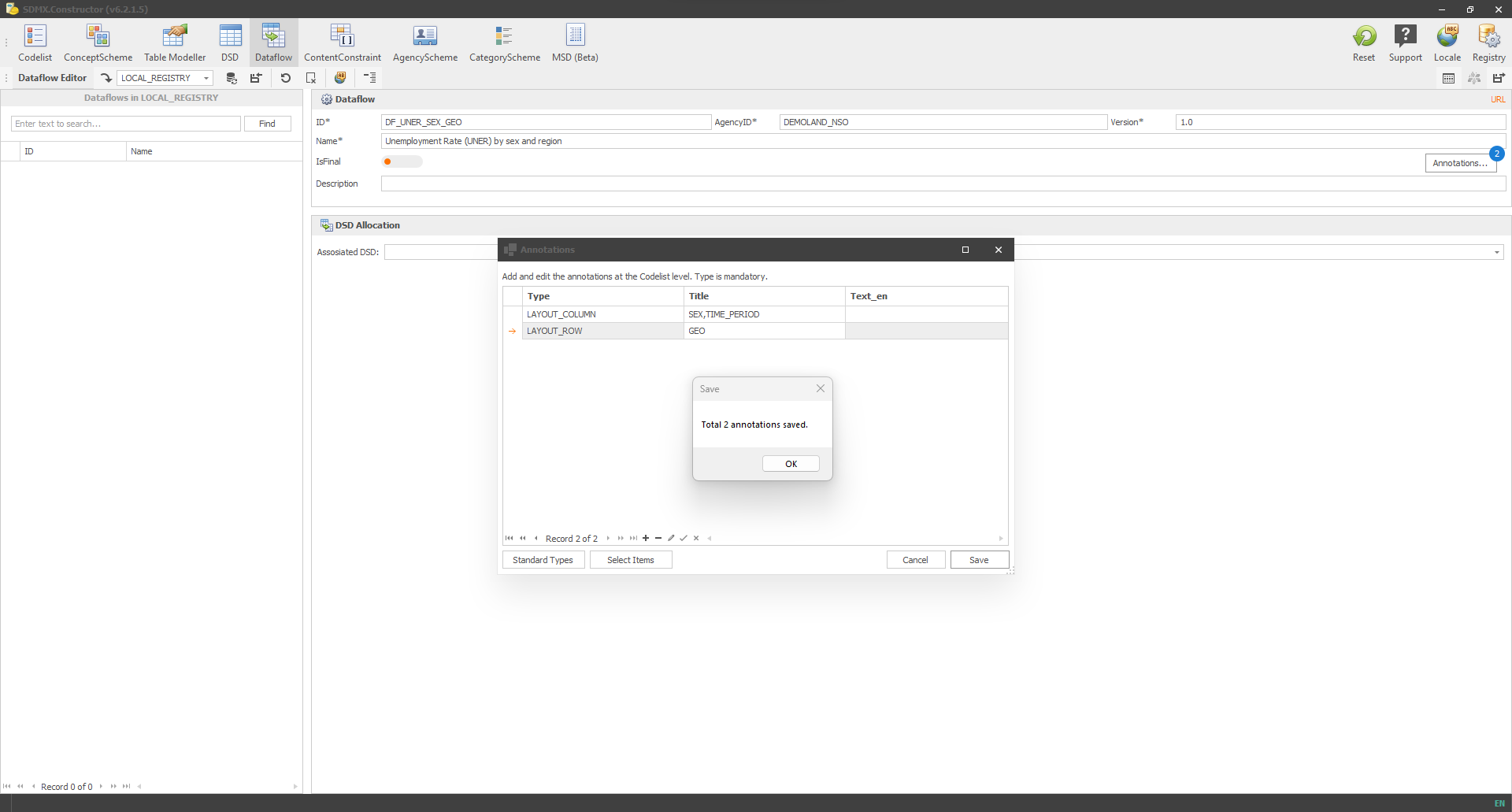 Click here to enlarge the image
- Click OK. It will now show the 2 annotation notifications as highlighted below.
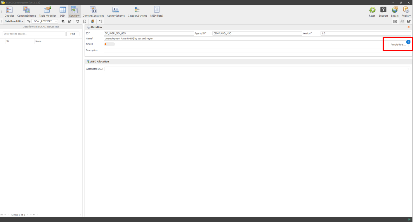 Click here to enlarge the image
- Now, in the DSD Allocation pane, in the Associated DSD dropdown, select the DSD on which this Dataflow will be based. We selected the DSD we created before - DEMOLAND_NSO:DSD_DEMOLAND_NSO(1.0).
 Click here to enlarge the image
- Now click on the Export/Save button, as shown below and click on Save.
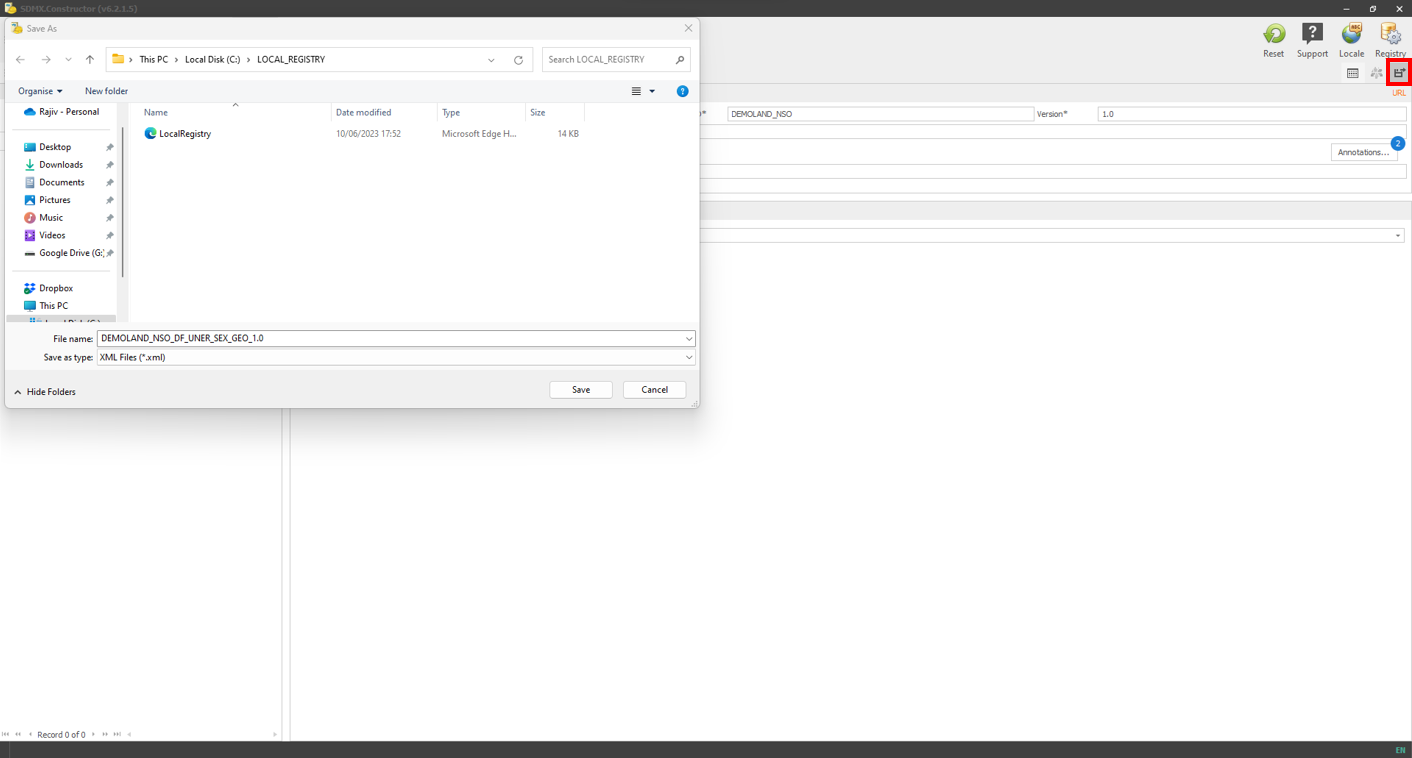 Click here to enlarge the image
- It will show a message as shown below.
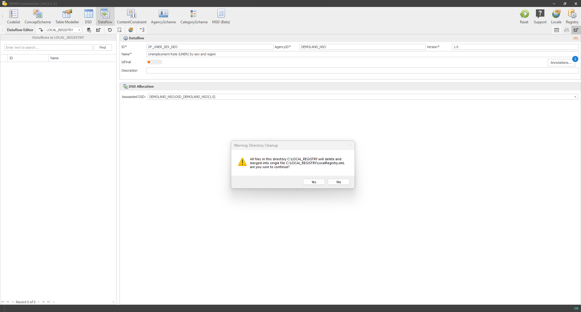 Click here to enlarge the image
- Clicking on Yes will show a message indicating that the XML file (containing the Dataflow) has been created.
 Click here to enlarge the image
- After that, you will see the XML file created if you go to the file’s location.
Creating ContentConstraint
- Click on the ContentConstraint button in the Editor menu and ensure that the folder we created before, LOCAL_REGISTRY, is selected from the ‘Load from registry’ dropdown option, as shown below.
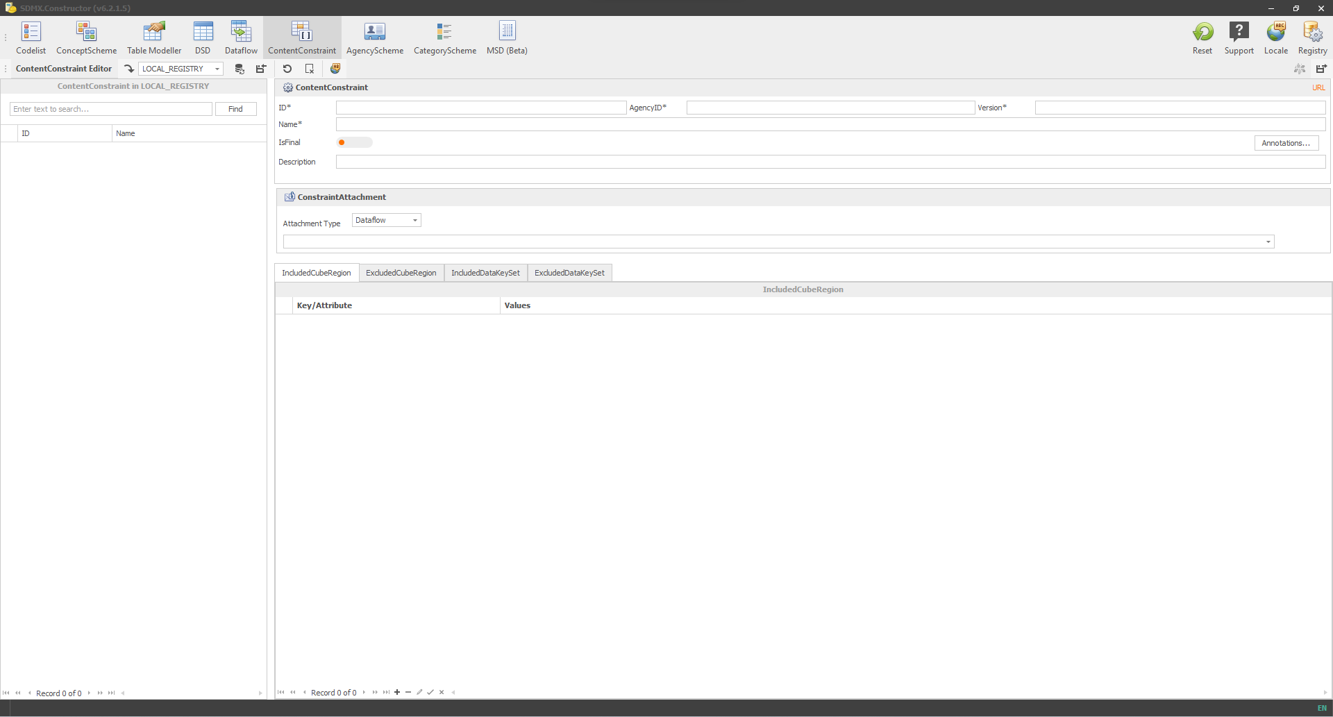 Click here to enlarge the image
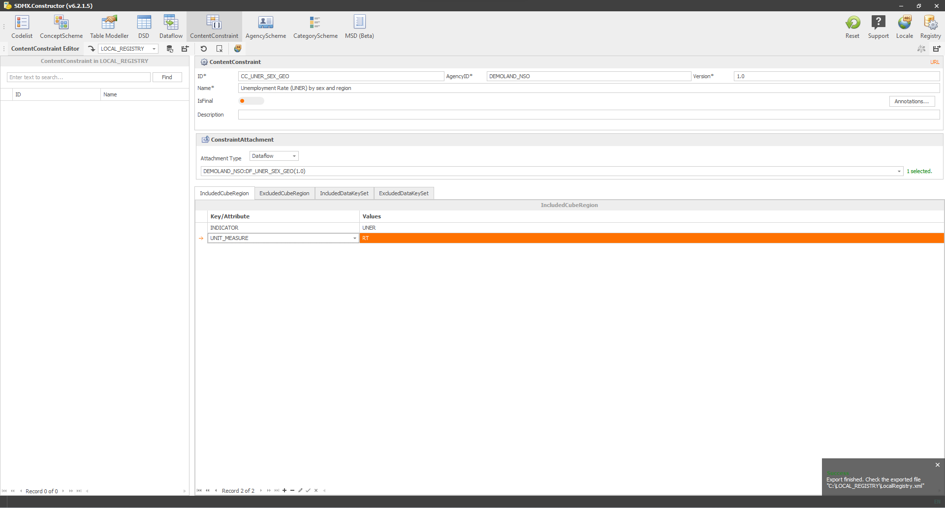
- Fill in the details for the ContentConstraint (ID = CC_UNER_SEX_GEO, AgencyID = DEMOLAND_NSO, Version = 1.0 and Name = Unemployment Rate (UNER) by sex and region) as shown below.
 Click here to enlarge the image
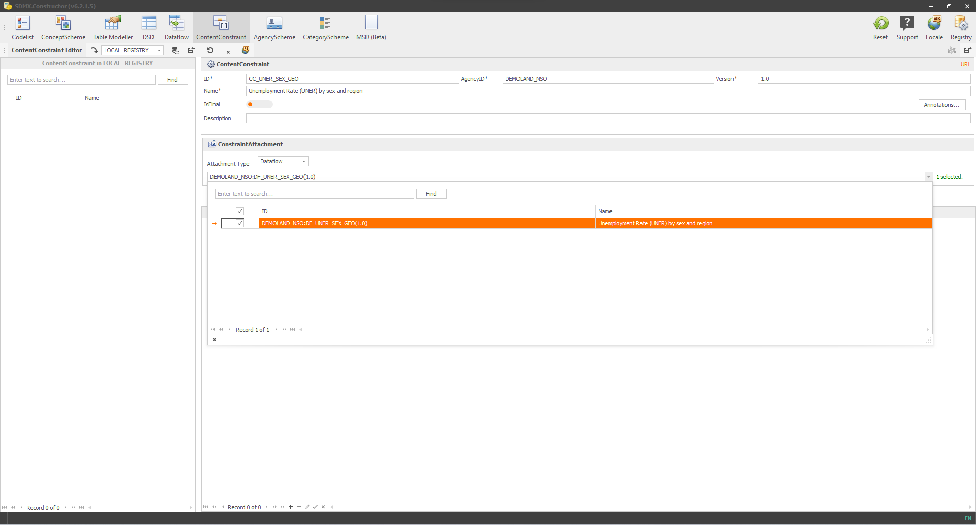
- Then in the ConstraintAttachment pane, in the Attachment Type, select the Dataflow option and from the dropdown list underneath, select the relevant dataflow as shown below.
 Click here to enlarge the image
- Then click the append (or +) button to add the required rows.
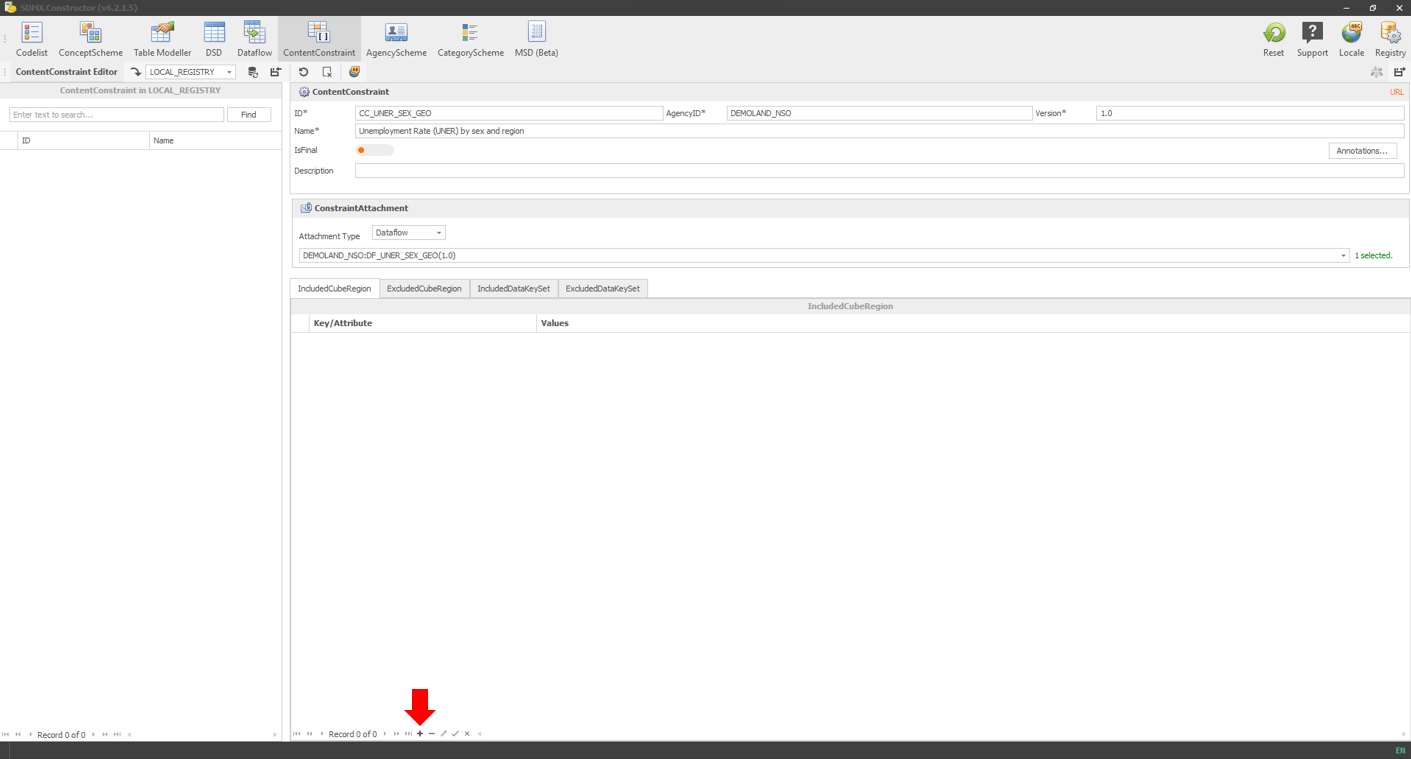 Click here to enlarge the image
- We add two rows. In the first row, we select the concept ‘Indicator’ and the value as UNER (for Unemployment Rate). In the second row, we select the concept ‘UNIT_Measure’ (for Unit of Measurement) and the value as RT (for Rate), as shown below.
 Click here to enlarge the image
- Now click on the Export/Save button, as shown below and click on Save in the resulting window.
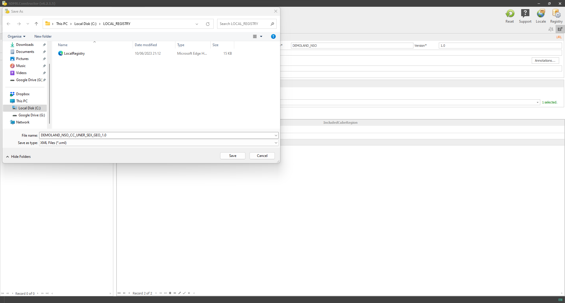 Click here to enlarge the image
- It will show a message as shown below.
 Click here to enlarge the image
Clicking on Yes will show a message in the bottom right-hand corner indicating that the XML file is created.
 Click here to enlarge the image
After that, you will see the XML file created if you go to the file’s location.
The Table Modeller approach
In SDMX Constructor, the Table Modeller feature (Under special topics, the functionality of the Table Modeller is detailed) provides an intuitive user interface for designing statistical tables and generating the corresponding SDMX artefacts in one go.
Recalling our two initial tables (Table: 4.1 and Table: 4.2), we will now generate DSDs, ContentConstraints and Dataflows. We can create all these artefacts through the Table Modeller option in the SDMX Constructor.
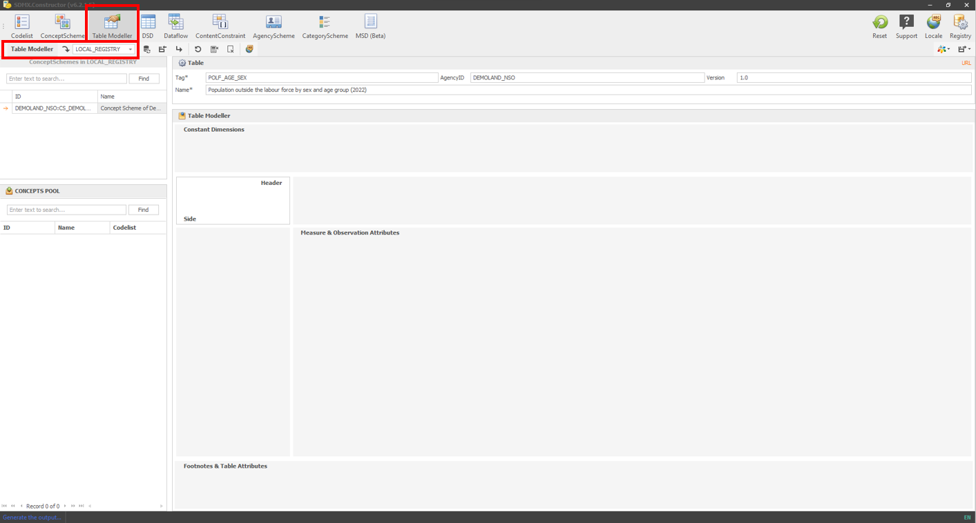
- Click on the Table Modeller button on top and ensure that the folder we created before, LOCAL_REGISTRY, is selected from the Table Modeller Editor’s ‘Load from registry’ dropdown option, as shown below.
 Click here to enlarge the image
- You will notice the concept scheme we created before, as highlighted below.
 Click here to enlarge the image
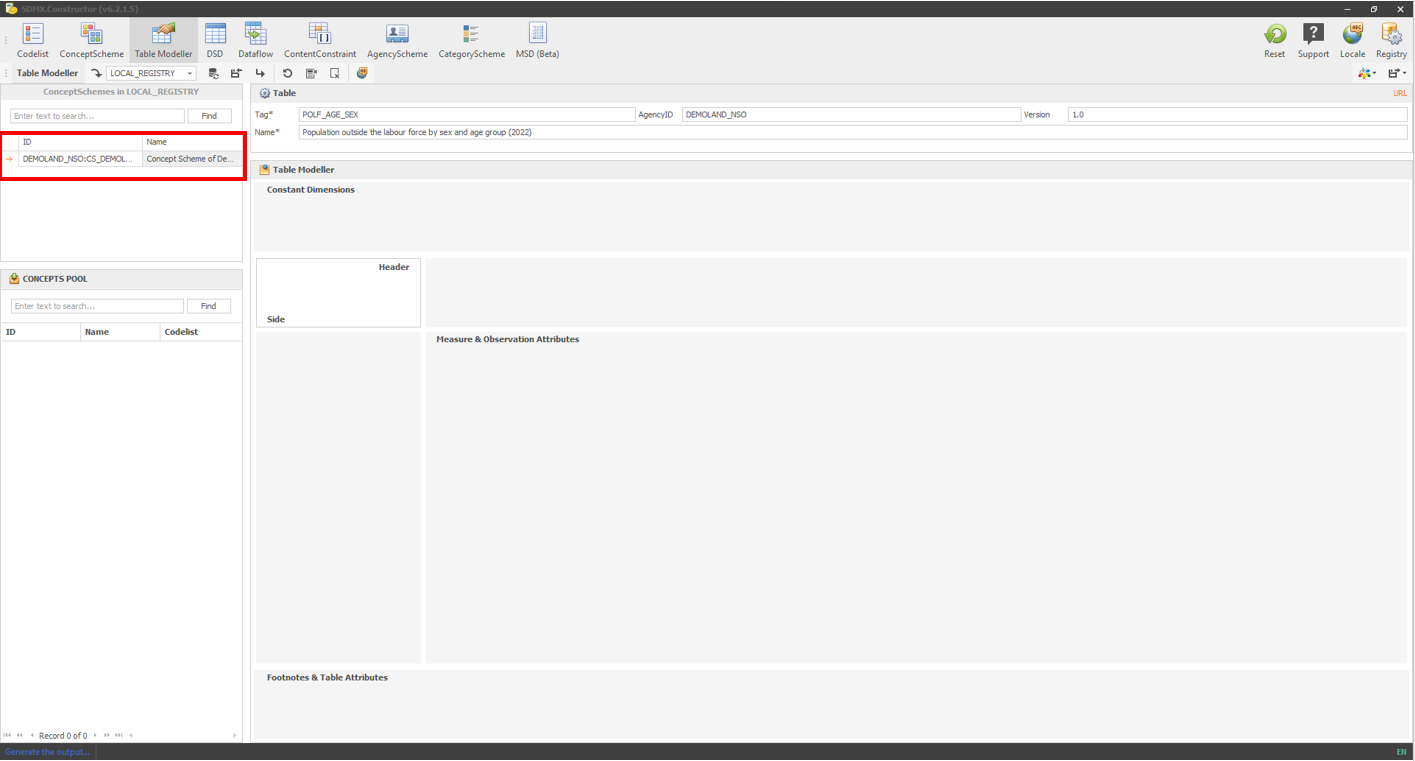
- Double-clicking the concept scheme will move it to the CONCEPT POOL, as shown below.
 Click here to enlarge the image
Now, you can select the concepts in the CONCEPT POOL, then drag and drop them into various spaces (Constant Dimensions, Header, Side, Measures & Observation Attributes and Footnotes & Table Attributes) on the right pane. The logic driving where to drop each concept comes from our original tables (Table: 4.1 and Table: 4.2).
For Table 4.1 (Unemployment Rate by sex and region), the following distribution will be representative.
 Click here to enlarge the image
- We can now apply two constraints: one for the indicator’s name and the other for the unit of measure. The indicator’s name will be the Unemployment Rate, which we can select by double-clicking the moved indicator concept as shown below.
 Click here to enlarge the image
- Another constraint would be the unit of measure. Because it is ‘rate’ (for Table 4.1), double-clicking the moved unit of measure concept would offer the option to select the rate. Select the Rate as shown below.
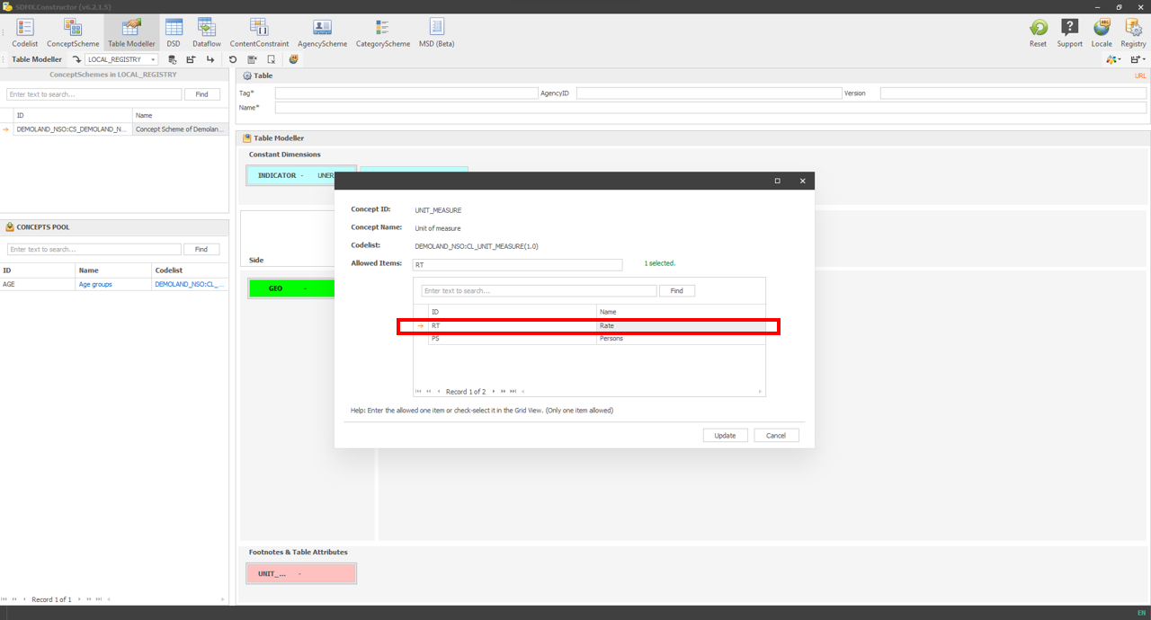 Click here to enlarge the image
- Now we add the table information as shown below.
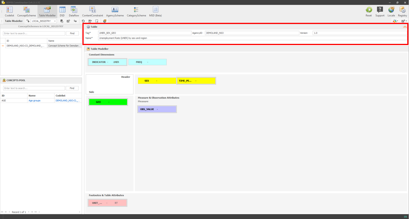 Click here to enlarge the image
- Then we will hit save (select ‘Save without descendants’), as shown below.
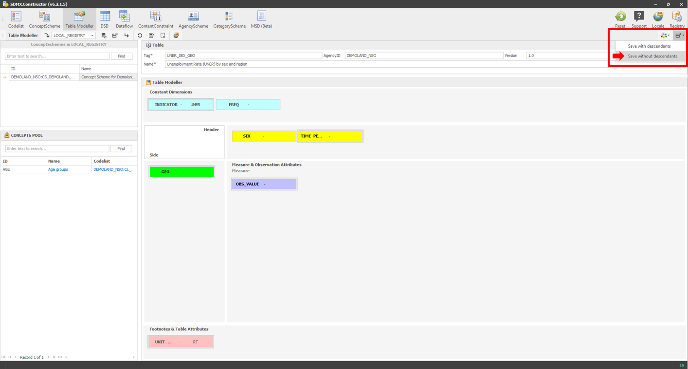 Click here to enlarge the image
- After saving, it will show a message as shown below.
 Click here to enlarge the image
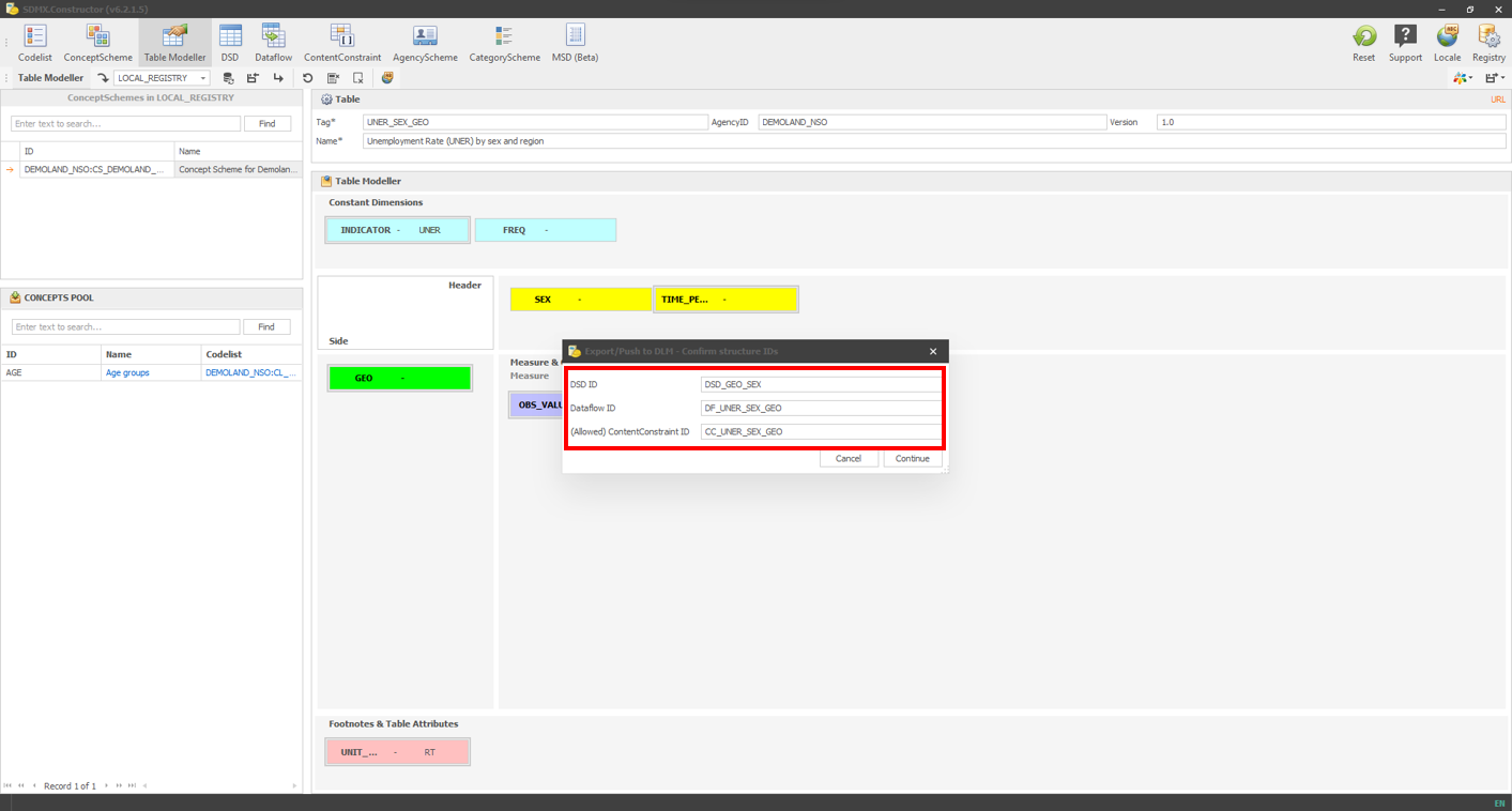
- Clicking on Continue will result in a pop-up asking to save the file, as shown below.
 Click here to enlarge the image
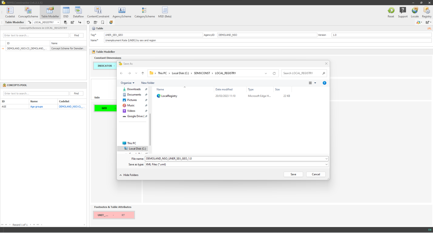
- Clicking Save will show this message and ask if the files should be merged.
 Click here to enlarge the image
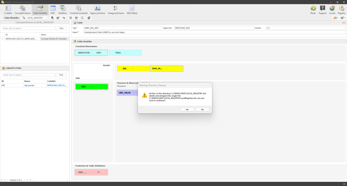
- Clicking on Yes will merge the file.
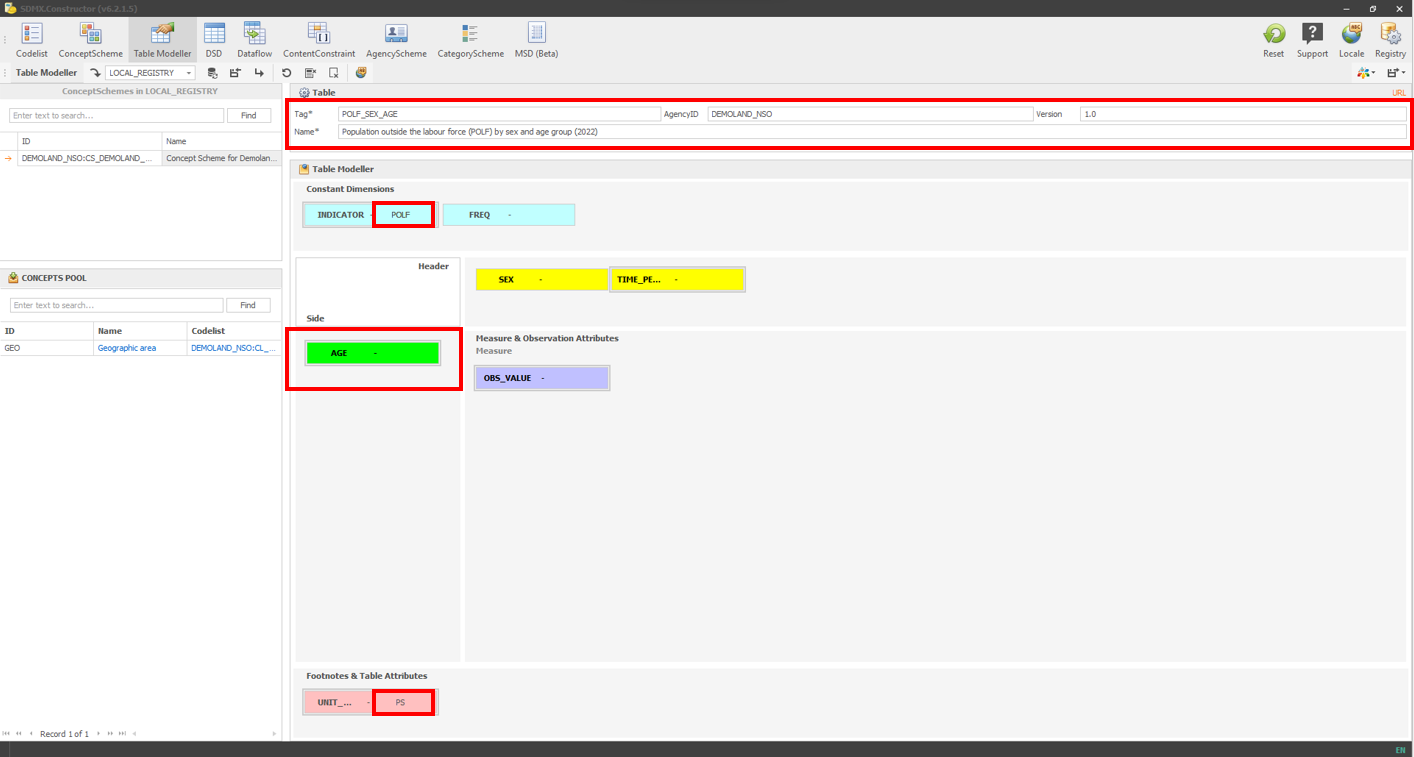
- We will repeat the process for Table 4.2 (Population outside the labour force by sex and age group (2022)). We can do that by moving Age to the ‘Side’ space (and removing the Geo back to the CONCEPT POOL), changing the constraints for the indicator to ‘Population outside the labour force’ and unit of measure to ‘Persons’, and updating the table information as shown below.
 Click here to enlarge the image
- After hitting the save (Save without descendants) button, the message will read like the one below.
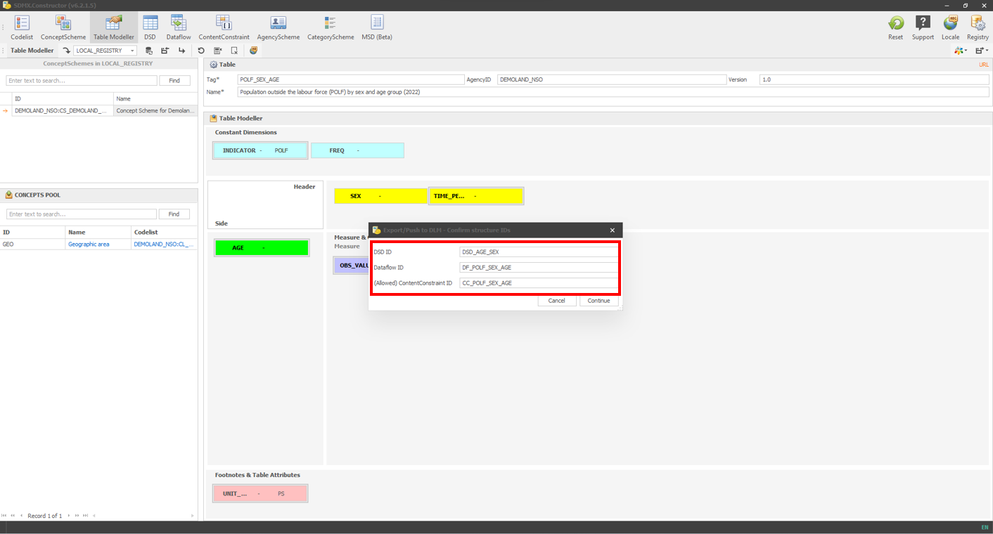 Click here to enlarge the image
Proceed with ‘Continue’, ‘Save’, and ‘Yes’ for merge.
We should see two DSDs, two content constraints and two data flows.
Remember, dataflows are the filtered view of the DSDs.